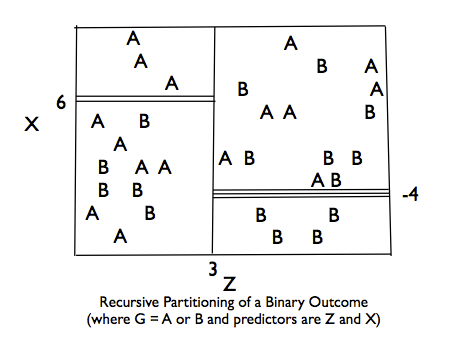
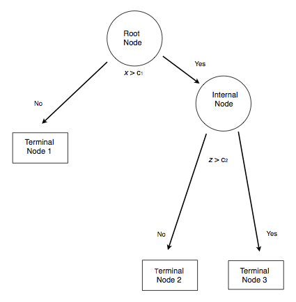
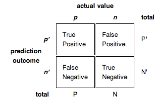
Classification and Regression Trees

class: center, middle, inverse, title-slide

# Classification and Regression Trees
## 
### Jason Bryer, Ph.D.
### 2024-11-04

---
# Classification and Regression Trees

The goal of CART methods is to find best predictor in X of some outcome, y. CART methods do this recursively using the following procedures:

* Find the best predictor in X for y.
* Split the data into two based upon that predictor.
* Repeat 1 and 2 with the split data sets until a stopping criteria has been reached.

There are a number of possible stopping criteria including: Only one data point remains.

* All data points have the same outcome value.
* No predictor can be found that sufficiently splits the data.

---
# Recursive Partitioning Logic of CART

.pull-left[
Consider the scatter plot to the right with the following characteristics:

* Binary outcome, G, coded “A” or “B”.
* Two predictors, x and z
* The vertical line at z = 3 creates the first partition.
* The double horizontal line at x = -4 creates the second partition.
* The triple horizontal line at x = 6 creates the third partition.
]
.pull-right[
![](images/Partitioning.png)
]

---
# Tree Structure

.pull-left[
* The root node contains the full data set.
* The data are split into two mutually exclusive pieces. Cases where x > ci go to the right, cases where x <= ci go to the left.
* Those that go to the left reach a terminal node.
* Those on the right are split into two mutually exclusive pieces. Cases where z > c2 go to the right and terminal node 3; cases where z <= c2 go to the left and terminal node 2.
]
.pull-right[
![](images/TreeDiagram.png)
]

---
# Sum of Squared Errors

The sum of squared errors for a tree *T* is:

`$$S=\sum _{ c\in leaves(T) }^{  }{ \sum _{ i\in c }^{  }{ { (y-{ m }_{ c }) }^{ 2 } }  }$$`

Where, `${ m }_{ c }=\frac { 1 }{ n } \sum _{ i\in c }^{  }{ { y }_{ i } }$`, the prediction for leaf \textit{c}.

Or, alternatively written as:

`$$S=\sum _{ c\in leaves(T) }^{  }{ { n }_{ c }{ V }_{ c } }$$`

Where `$V_{c}$` is the within-leave variance of leaf \textit{c}.

Our goal then is to find splits that minimize S.

---
# Advantages of CART Methods

* Making predictions is fast.

* It is easy to understand what variables are important in making predictions.

* Trees can be grown with data containing missingness. For rows where we cannot reach a leaf node, we can still make a prediction by averaging the leaves in the sub-tree we do reach.

* The resulting model will inherently include interaction effects. There are many reliable algorithms available.

---
# Regression Trees

In this example we will predict the median California house price from the house’s longitude and latitude.

``` r
str(calif)
```

```
## 'data.frame':	20640 obs. of  10 variables:
##  $ MedianHouseValue: num  452600 358500 352100 341300 342200 ...
##  $ MedianIncome    : num  8.33 8.3 7.26 5.64 3.85 ...
##  $ MedianHouseAge  : num  41 21 52 52 52 52 52 52 42 52 ...
##  $ TotalRooms      : num  880 7099 1467 1274 1627 ...
##  $ TotalBedrooms   : num  129 1106 190 235 280 ...
##  $ Population      : num  322 2401 496 558 565 ...
##  $ Households      : num  126 1138 177 219 259 ...
##  $ Latitude        : num  37.9 37.9 37.9 37.9 37.9 ...
##  $ Longitude       : num  -122 -122 -122 -122 -122 ...
##  $ cut.prices      : Factor w/ 4 levels "[1.5e+04,1.2e+05]",..: 4 4 4 4 4 4 4 3 3 3 ...
```

---
# Tree 1

``` r
treefit <- tree(log(MedianHouseValue) ~ Longitude + Latitude, data=calif)
plot(treefit); text(treefit, cex=0.75)
```

---
# Tree 1

---
# Tree 1

``` r
summary(treefit)
```

```
## 
## Regression tree:
## tree(formula = log(MedianHouseValue) ~ Longitude + Latitude, 
##     data = calif)
## Number of terminal nodes:  12 
## Residual mean deviance:  0.1662 = 3429 / 20630 
## Distribution of residuals:
##     Min.  1st Qu.   Median     Mean  3rd Qu.     Max. 
## -2.75900 -0.26080 -0.01359  0.00000  0.26310  1.84100
```

Here “deviance” is the mean squared error, or root-mean-square error of `$\sqrt{.166} =  0.41$`.

---
# Tree 2, Reduce Minimum Deviance

We can increase the fit but changing the stopping criteria with the mindev parameter.

``` r
treefit2 <- tree(log(MedianHouseValue) ~ Longitude + Latitude, data=calif, mindev=.001)
summary(treefit2)
```

```
## 
## Regression tree:
## tree(formula = log(MedianHouseValue) ~ Longitude + Latitude, 
##     data = calif, mindev = 0.001)
## Number of terminal nodes:  68 
## Residual mean deviance:  0.1052 = 2164 / 20570 
## Distribution of residuals:
##     Min.  1st Qu.   Median     Mean  3rd Qu.     Max. 
## -2.94700 -0.19790 -0.01872  0.00000  0.19970  1.60600
```

With the larger tree we now have a root-mean-square error of 0.32.

---
# Tree 2, Reduce Minimum Deviance

---
# Tree 3, Include All Variables

However, we can get a better fitting model by including the other variables.

``` r
treefit3 <- tree(log(MedianHouseValue) ~ ., data=calif)
summary(treefit3)
```

```
## 
## Regression tree:
## tree(formula = log(MedianHouseValue) ~ ., data = calif)
## Variables actually used in tree construction:
## [1] "cut.prices"
## Number of terminal nodes:  4 
## Residual mean deviance:  0.03608 = 744.5 / 20640 
## Distribution of residuals:
##      Min.   1st Qu.    Median      Mean   3rd Qu.      Max. 
## -1.718000 -0.127300  0.009245  0.000000  0.130000  0.358600
```

With all the available variables, the root-mean-square error is 0.11.

---
# Classification Trees

* `pclass`: Passenger class (1 = 1st; 2 = 2nd; 3 = 3rd)
* `survival`: A Boolean indicating whether the passenger survived or not (0 = No; 1 = Yes); this is our target
* `name`: A field rich in information as it contains title and family names
* `sex`: male/female
* `age`: Age, a significant portion of values are missing
* `sibsp`: Number of siblings/spouses aboard
* `parch`: Number of parents/children aboard
* `ticket`: Ticket number.
* `fare`: Passenger fare (British Pound).
* `cabin`: Does the location of the cabin influence chances of survival?
* `embarked`: Port of embarkation (C = Cherbourg; Q = Queenstown; S = Southampton)
* `boat`: Lifeboat, many missing values
* `body`: Body Identification Number
* `home.dest`: Home/destination

---
# Classification using `rpart`

``` r
(titanic.rpart <- rpart(survived ~ pclass + sex + age + sibsp,
   data=titanic.train))
```

```
## n= 981 
## 
## node), split, n, deviance, yval
##       * denotes terminal node
## 
## 1) root 981 231.65140 0.3822630  
##   2) sex=male 636  97.35849 0.1886792  
##     4) pclass>=1.5 504  64.53968 0.1507937  
##       8) age>=3.5 489  57.82004 0.1370143 *
##       9) age< 3.5 15   3.60000 0.6000000 *
##     5) pclass< 1.5 132  29.33333 0.3333333 *
##   3) sex=female 345  66.52174 0.7391304  
##     6) pclass>=2.5 150  37.44000 0.4800000 *
##     7) pclass< 2.5 195  11.26154 0.9384615 *
```

---
# Classification using `rpart`

``` r
plot(titanic.rpart); text(titanic.rpart, use.n=TRUE, cex=1)
```

---
# Classification using `ctree`

``` r
(titanic.ctree <- ctree(survived ~ pclass + sex + age + sibsp, data=titanic.train))
```

```
## 
## 	 Conditional inference tree with 7 terminal nodes
## 
## Response:  survived 
## Inputs:  pclass, sex, age, sibsp 
## Number of observations:  981 
## 
## 1) sex == {female}; criterion = 1, statistic = 286.705
##   2) pclass <= 2; criterion = 1, statistic = 83.519
##     3)*  weights = 195 
##   2) pclass > 2
##     4) sibsp <= 1; criterion = 0.98, statistic = 7.833
##       5)*  weights = 129 
##     4) sibsp > 1
##       6)*  weights = 21 
## 1) sex == {male}
##   7) pclass <= 1; criterion = 0.999, statistic = 13.94
##     8)*  weights = 132 
##   7) pclass > 1
##     9) age <= 3; criterion = 1, statistic = 15.936
##       10)*  weights = 15 
##     9) age > 3
##       11) age <= 32; criterion = 0.961, statistic = 6.666
##         12)*  weights = 358 
##       11) age > 32
##         13)*  weights = 131
```

---
# Classification using `ctree`

``` r
plot(titanic.ctree)
```

---
# Receiver Operating Characteristic (ROC) Graphs

.pull-left[
In a classification model, outcomes are either as positive (*p*) or negative (*n*). There are then four possible outcomes:

* **true positive** (TP) The outcome from a prediction is *p* and the actual value is also *p*.
* **false positive** (FP) The actual value is *n*.
* **true negative** (TN) Both the prediction outcome and the actual value are *n*.
* **false negative** (FN) The prediction outcome is *n* while the actual value is *p*.

]
.pull-right[
![](images/rocdiagram.png)
]

---
# ROC Curve

.center[
![](images/ROCspace.png)
]

---
# Ensemble Methods

Ensemble methods use multiple models that are combined by weighting, or averaging, each individual model to provide an overall estimate. Each model is a random sample of the sample. Common ensemble methods include:

* *Boosting* - Each successive trees give extra weight to points incorrectly predicted by earlier trees. After all trees have been estimated, the prediction is determined by a weighted “vote” of all predictions (i.e. results of each individual tree model).

* *Bagging* - Each tree is estimated independent of other trees. A simple “majority vote” is take for the prediction.

* *Random Forests* - In addition to randomly sampling the data for each model, each split is selected from a random subset of all predictors.

* *Super Learner* - An ensemble of ensembles. See https://cran.r-project.org/web/packages/SuperLearner/vignettes/Guide-to-SuperLearner.html

---
class: font90
# Random Forests

The random forest algorithm works as follows:

1. Draw `$n_{tree}$` bootstrap samples from the original data.

2. For each bootstrap sample, grow an unpruned tree. At each node, randomly sample `$m_{try}$` predictors and choose the best split among those predictors selected<footnote>Bagging is a special case of random forests where `$m_{try} = p$` where *p* is the number of predictors</footnote>.

3. Predict new data by aggregating the predictions of the ntree trees (majority votes for classification, average for regression).

Error rates are obtained as follows:

1. At each bootstrap iteration predict data not in the bootstrap sample (what Breiman calls “out-of-bag”, or OOB, data) using the tree grown with the bootstrap sample.

2. Aggregate the OOB predictions. On average, each data point would be out-of-bag 36% of the times, so aggregate these predictions. The calculated error rate is called the OOB estimate of the error rate.

---
# Random Forests: Titanic

``` r
titanic.rf <- randomForest(factor(survived) ~ pclass + sex + age + sibsp,
						   data = titanic.train,
						   ntree = 5000,
						   importance = TRUE)
```

``` r
importance(titanic.rf)
```

```
##                0          1 MeanDecreaseAccuracy MeanDecreaseGini
## pclass  88.81141  65.808147            104.86923         45.09446
## sex    246.26889 300.826634            311.78582        129.85968
## age     88.49288  -1.666373             81.77633         55.43950
## sibsp   71.87125 -21.177906             50.98780         16.45040
```

---
# Random Forests: Titanic (cont.)

``` r
importance(titanic.rf)
```

---
# Random Forests: Titanic

``` r
min_depth_frame <- min_depth_distribution(titanic.rf)
```

``` r
plot_min_depth_distribution(min_depth_frame)
```

---
# Which model to use?

Fernández-Delgado et al (2014) evaluated 179 classifiers across 121 data sets. They found that, on average, random forest performs the best achieving 94% of the maximum overcoming 90% in the 84.3% of the data sets

https://jmlr.org/papers/volume15/delgado14a/delgado14a.pdf

If you are interested in this topic, I have been working on a R package that creates a framework to evaluate predictive models across data sets for both classificaiton and regression.

https://github.com/jbryer/mldash

---
class: left, font140
# One Minute Paper

.pull-left[
1. What was the most important thing you learned during this class?
2. What important question remains unanswered for you?
]
.pull-right[
<img src="CART-Methods_files/figure-html/unnamed-chunk-15-1.png" style="display: block; margin: auto;" />
]

https://forms.gle/U4UXAosdjHorxY919